
Why Time in the Market Beats Timing the Market: A Deep Dive into Dollar-Cost Averaging vs. Lump Sum Investing
Introduction
When it comes to investing, the debate often centers on whether it’s better to invest all your money at once (lump sum investing) or to spread your investments over time (Dollar-Cost Averaging or DCA). While both strategies have their merits, historical data from the S&P 500 suggests that staying invested for the long term is crucial. This article explores the performance of these two strategies over various time horizons, reinforcing the principle that time in the market beats timing the market.
Understanding the Strategies
What is Dollar-Cost Averaging (DCA)?
Dollar-Cost Averaging (DCA) involves investing a fixed amount of money at regular intervals, regardless of market conditions. This strategy helps mitigate the risk of entering the market at the wrong time and allows investors to purchase more shares when prices are low and fewer when prices are high, reducing the average cost per share over time.
What is Lump Sum Investing?
Lump sum investing, on the other hand, is the strategy of investing all your available funds at once. While this approach can yield higher returns if the market performs well, it also exposes the investor to the risk of a significant market downturn immediately after investing.
The Historical Perspective
A Look Back: S&P 500 Performance Over Time
The S&P 500 has historically provided strong returns, despite periods of volatility. To understand the impact of different investment strategies, we analyzed historical data, considering various investment horizons ranging from 5 to 35 years.
Simulating Investment Strategies: DCA vs. Lump Sum
Methodology: How We Ran the Simulation
We conducted simulations using historical S&P 500 data to compare the performance of DCA and Lump Sum strategies over different time horizons. We simulated a consistent monthly investment of $500 for DCA and a one-time investment of the same total amount for Lump Sum. Investment horizons tested include 5, 7, 10, 15, 20, 25, and 35 years.
import pandas as pd
import numpy as np
import yfinance as yf
from datetime import timedelta, datetime
import matplotlib.pyplot as plt

# Download S&P 500 historical data
df = yf.download('^SPX', start='1900-01-01')
spy = df[['Close']].resample('D').ffill().rename(columns={'Close': 'price'})
spy = spy.resample('MS').last()

# Parameters
MONTHLY_INVESTMENT = 500
HORIZONS = [5, 7, 10, 15, 20, 25, 35]  # Different investment horizons in years
dates = spy.index

def create_fanchart(arr, ax, color='blue'):
    x = np.arange(arr.shape[0])
    # for the median use `np.median` and change the legend below
    mean = np.mean(arr, axis=1)
    offsets = (10, 20, 30, 40)

    ax.plot(mean, color='black', lw=2)
    for offset in offsets:
        low = np.percentile(arr, 50-offset, axis=1)
        high = np.percentile(arr, 50+offset, axis=1)
        # since `offset` will never be bigger than 50, do 55-offset so that
        # even for the whole range of the graph the fanchart is visible
        alpha = (55 - offset) / 100
        ax.fill_between(x, low, high, color=color, alpha=alpha)
    ax.legend(['Mean'] + [f'Pct{2*o}' for o in offsets])
    return ax

# Function to simulate DCA strategy for different horizons
def sim_dca(horizon, start_date):
    dates_in_sim = dates[(dates >= start_date) & (dates < start_date + timedelta(horizon * 365))]
    investments = [{'date': date,
                    'money_spent': MONTHLY_INVESTMENT,
                    'quantity_bought': MONTHLY_INVESTMENT / spy.loc[date].price}
                   for date in dates_in_sim]

    invest_df = pd.DataFrame(investments).set_index('date')
    invest_df['tt_qty'] = invest_df['quantity_bought'].cumsum()
    invest_df['index_price'] = spy['price'].reindex(invest_df.index)
    invest_df['market_value'] = invest_df['index_price'] * invest_df['tt_qty']
    invest_df['total_money_spent'] = invest_df['money_spent'].cumsum()


    return invest_df

# Function to calculate statistics for different horizons
def calculate_statistics(horizon):
    mc = []
    dca_results = []
    lumsum_results = []
    for start_date in dates[dates < dates.max() - timedelta(horizon * 365)]:
        invest_df = sim_dca(horizon, start_date)
        benefit_strategy = (invest_df['market_value'].iloc[-1] - invest_df['total_money_spent'].iloc[-1]) / invest_df['total_money_spent'].iloc[-1]
        lumpsum_benefit = (invest_df['total_money_spent'].iloc[-1] *
                           (invest_df['index_price'].iloc[-1] / invest_df['index_price'].iloc[0]) -
                           invest_df['total_money_spent'].iloc[-1]) / invest_df['total_money_spent'].iloc[-1]


        mc.append({'start_date': start_date,
                   'benefit_strategy': benefit_strategy,
                   'lumpsum_benefit': lumpsum_benefit})

        lumsum_results.append((spy.loc[invest_df['market_value'].index[0]: invest_df['market_value'].index[-1]].reset_index(drop=True)['price'].pct_change().fillna(0)+1).cumprod())
        dca_results.append(((invest_df['market_value'] / invest_df['total_money_spent']).reset_index(drop=True).pct_change().fillna(0)+1).cumprod())

    # Create subplots
    fig, (ax1, ax2) = plt.subplots(2, 1, figsize=(5, 6))  # 2 rows, 1 column

    # DCA results
    ax1 = create_fanchart(np.array(dca_results).T, ax1, color='blue')
    ax1.set_title(f"DCA Return for period {horizon} years")

    # Lumsum results
    ax2 = create_fanchart(np.array(lumsum_results).T, ax2, color='green')
    ax2.set_title(f'Lumpsum Return for period {horizon} years')

    plt.tight_layout()  # Adjust layout to prevent overlap
    plt.show()

    return pd.DataFrame(mc).set_index('start_date')

for horizon in HORIZONS:
    mc_df = calculate_statistics(horizon)
    stats = mc_df['benefit_strategy'].describe().to_dict()

    print(f"\n### Horizon: {horizon} Years ###")
    print(f'Average percentage gain using DCA: {stats["mean"]*100:.1f}%')
    print(f'Median percentage gain using DCA: {stats["50%"]*100:.1f}%')
    print(f'q25 percentage gain using DCA: {stats["25%"]*100:.1f}%')
    print(f'q75 percentage gain using DCA: {stats["75%"]*100:.1f}%')

    proba_of_losing_dca = len(mc_df[mc_df['benefit_strategy'] < 0]) / len(mc_df)
    print(f'Probability of losing money with DCA: {proba_of_losing_dca*100:.1f}%')

    stats = mc_df['lumpsum_benefit'].describe().to_dict()
    print(f'Average percentage gain using lumpsum: {stats["mean"]*100:.1f}%')
    print(f'Median percentage gain using lumpsum: {stats["50%"]*100:.1f}%')
    print(f'q25 percentage gain using lumpsum: {stats["25%"]*100:.1f}%')
    print(f'q75 percentage gain using lumpsum: {stats["75%"]*100:.1f}%')

    proba_of_losing_lumpsum = len(mc_df[mc_df['lumpsum_benefit'] < 0]) / len(mc_df)
    print(f'Probability of losing money with lumpsum: {proba_of_losing_lumpsum*100:.1f}%')
</div>
Results Breakdown: Analyzing Performance Across Different Horizons
5-Year Horizon
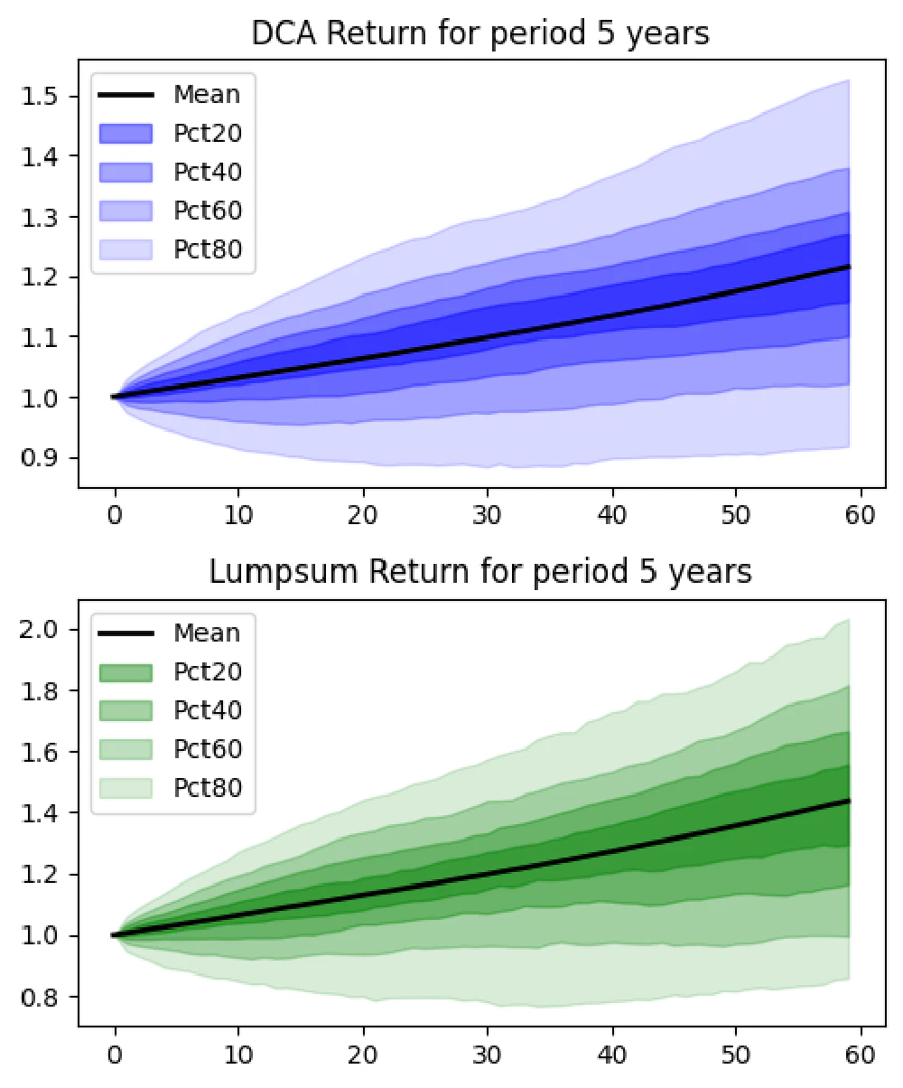
- DCA Results:
- Average gain: 21.5%
- Probability of loss: 17.2%
- Lump Sum Results:
- Average gain: 43.7%
- Probability of loss: 20.1%
Short-term horizons are more susceptible to market volatility. While Lump Sum showed higher average returns, it also had a higher risk of loss.
7-Year Horizon
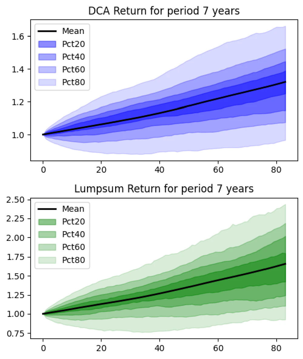
- DCA Results:
- Average gain: 32.0%
- Probability of loss: 12.3%
- Lump Sum Results:
- Average gain: 65.6%
- Probability of loss: 14.2%
With a 7-year horizon, both strategies perform better, but the probability of loss decreases significantly for DCA, showcasing its risk-mitigating benefits.
10-Year Horizon
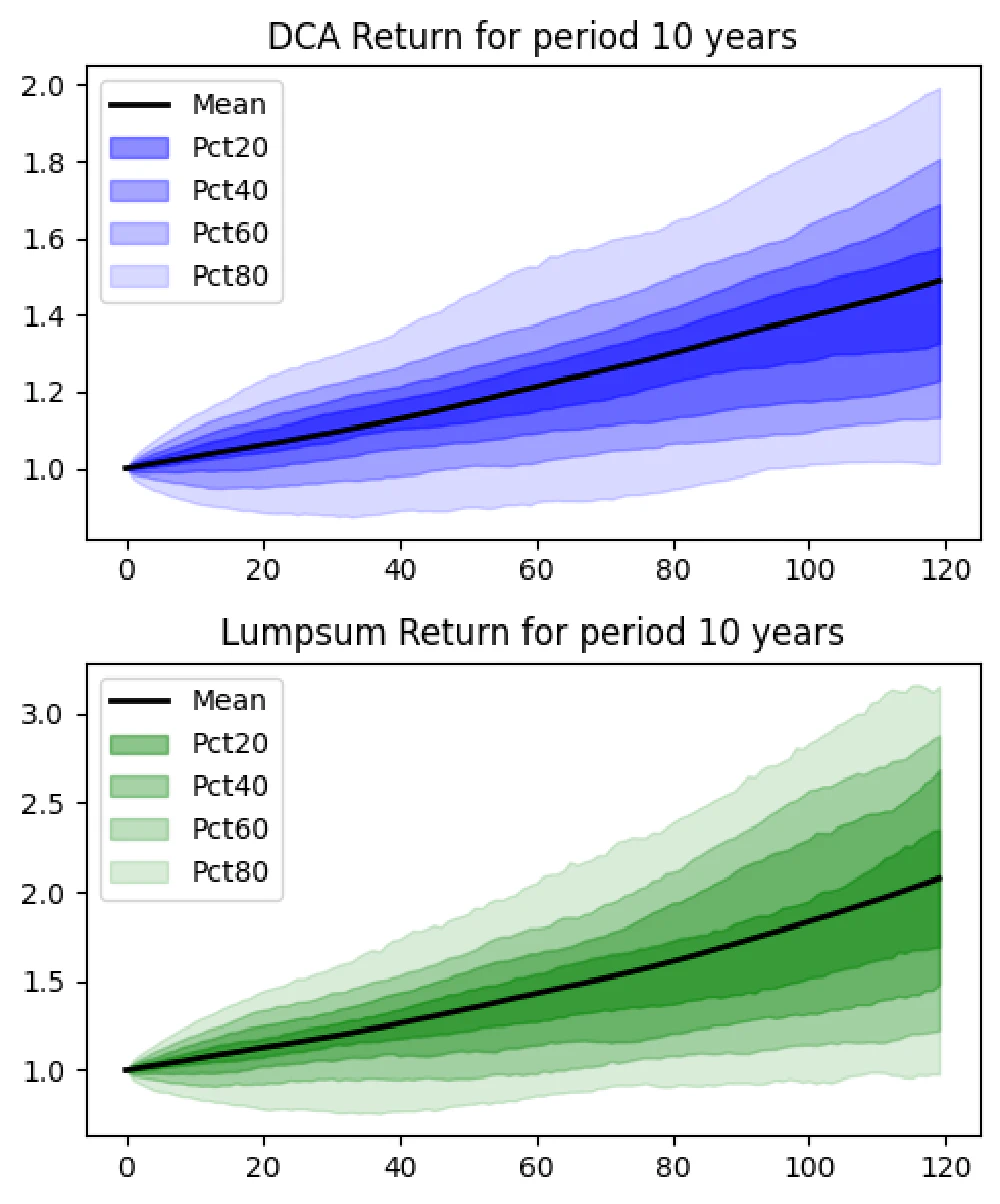
- DCA Results:
- Average gain: 49.0%
- Probability of loss: 8.7%
- Lump Sum Results:
- Average gain: 107.6%
- Probability of loss: 10.9%
At the 10-year mark, the probability of loss for both strategies falls below 10%. Lump Sum investing continues to outperform, but the risk reduction with DCA becomes evident.
15-Year Horizon
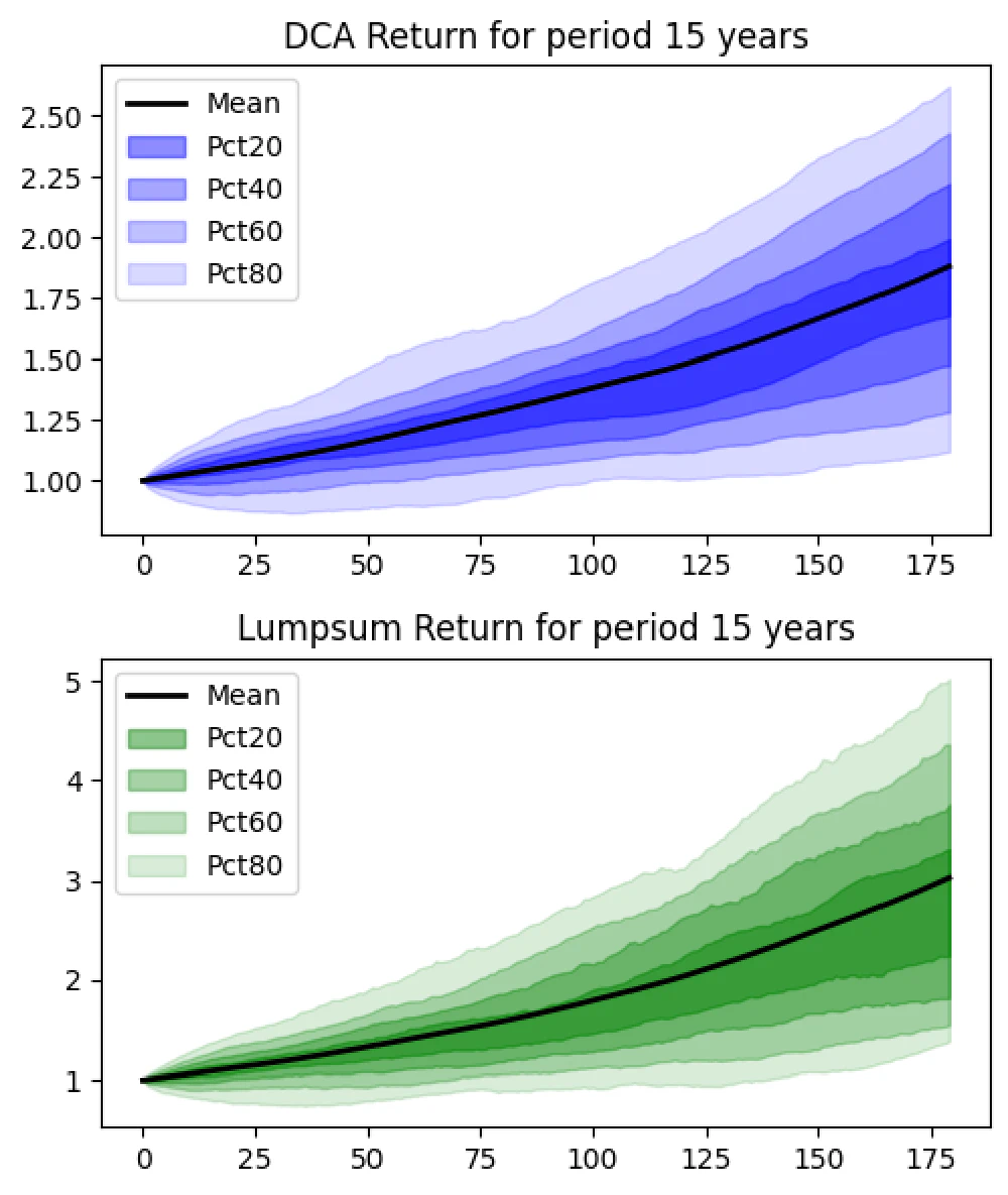
- DCA Results:
- Average gain: 88.0%
- Probability of loss: 2.7%
- Lump Sum Results:
- Average gain: 202.8%
- Probability of loss: 3.6%
Over 15 years, the benefits of being invested long-term become clearer. The risk of losing money with DCA is minimal, and Lump Sum sees substantial gains.
20-Year Horizon
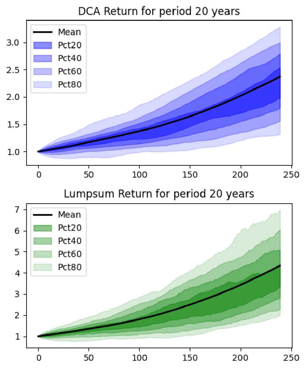
- DCA Results:
- Average gain: 137.4%
- Probability of loss: 0.2%
- Lump Sum Results:
- Average gain: 333.9%
- Probability of loss: 3.7%
With a 20-year horizon, both strategies show impressive gains, but the almost non-existent risk of loss with DCA demonstrates the importance of staying invested.
25-Year Horizon
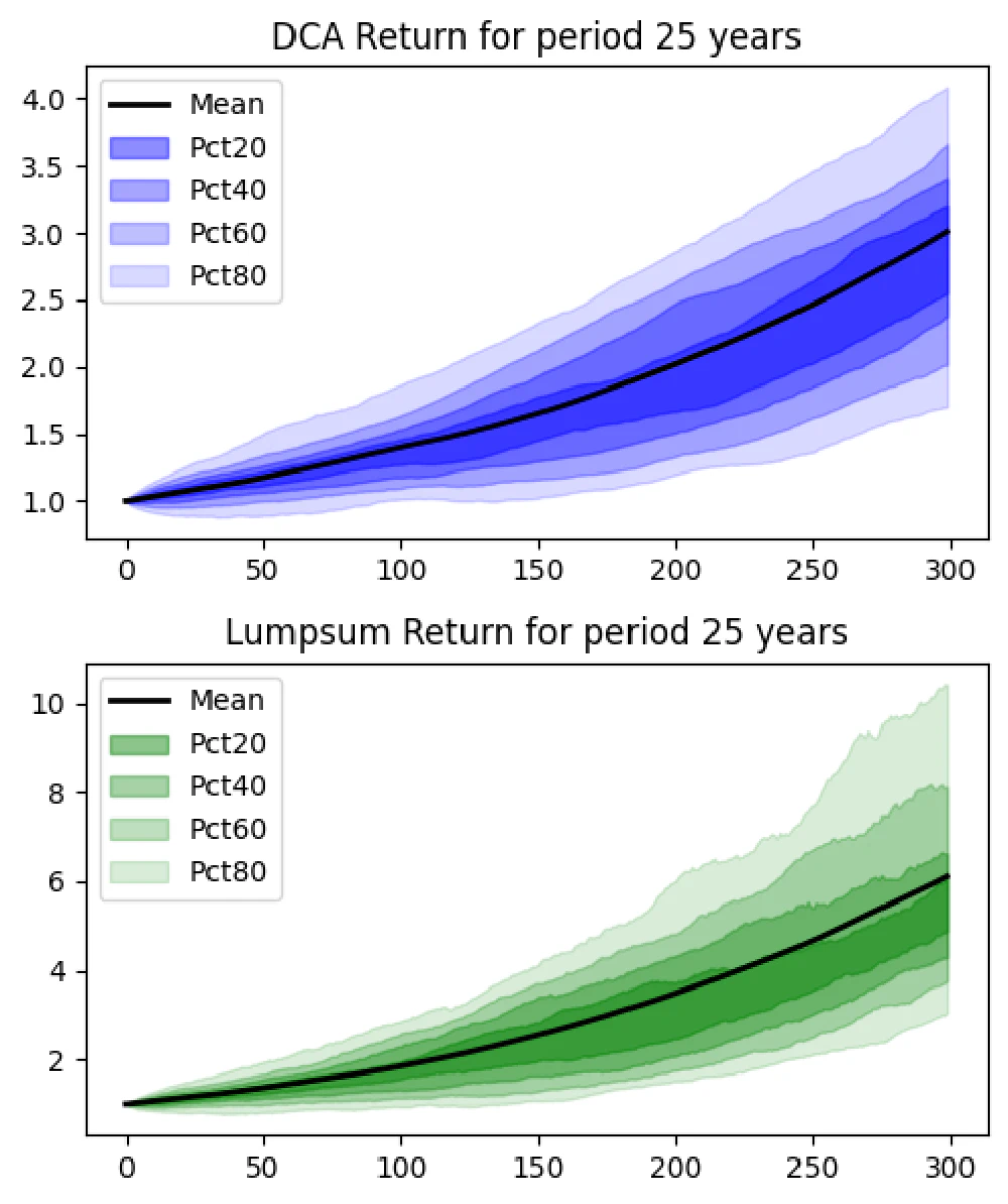
- DCA Results:
- Average gain: 200.9%
- Probability of loss: 0.0%
- Lump Sum Results:
- Average gain: 511.7%
- Probability of loss: 0.2%
Longer investment periods significantly reduce the risk of loss, and both strategies yield high returns, with Lump Sum still leading in average gains.
35-Year Horizon
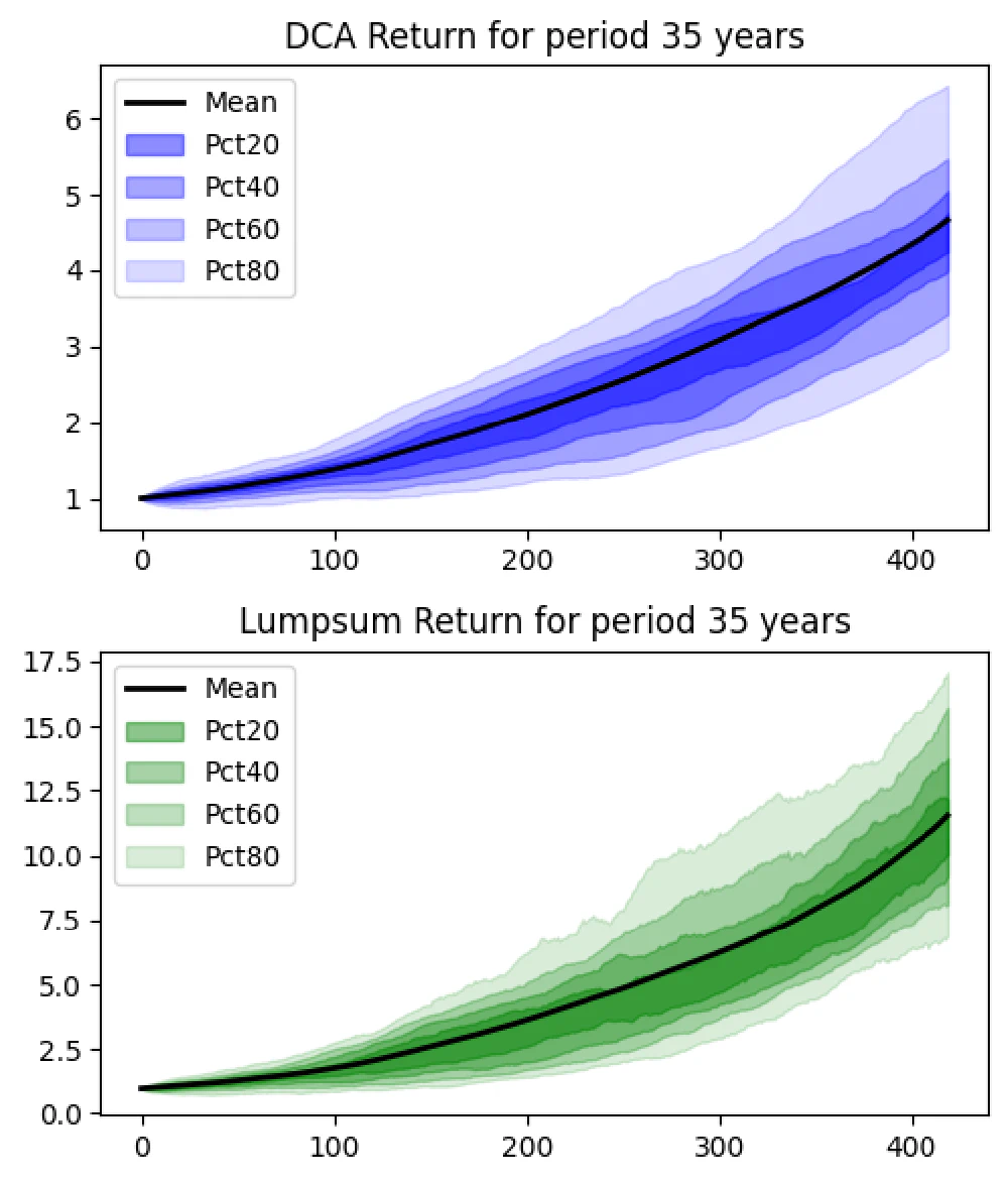
- DCA Results:
- Average gain: 366.6%
- Probability of loss: 0.0%
- Lump Sum Results:
- Average gain: 1052.5%
- Probability of loss: 0.0%
At 35 years, the risk of loss is eliminated, proving the strength of long-term investing. While Lump Sum yields higher returns, both strategies provide significant gains.
Key Insights from the Simulation
DCA: A Safer Approach to Investing?
DCA consistently shows lower risk and more stable returns, especially over shorter horizons. It’s a great strategy for investors who want to mitigate the risk of market volatility and build wealth steadily over time.
Lump Sum: Higher Returns But Higher Risk
Lump Sum investing tends to outperform DCA in terms of average returns, but it also carries a higher risk, particularly in shorter investment periods. For those confident in the timing of their investments, this strategy can be more rewarding.
Why Time in the Market Beats Timing the Market
Avoiding the Pitfalls of Market Timing
Trying to predict market highs and lows is a daunting task even for seasoned investors. The data supports the idea that it’s better to remain invested rather than trying to time the market.
The Power of Compound Growth
Over time, the growth of your investments compounds, leading to exponential gains. The longer you stay invested, the more time your money has to grow, underscoring why time in the market is so crucial.
Practical Tips for Investors
Start Early and Invest Consistently
The earlier you start investing, the more time your money has to compound. Setting up a regular investment plan, whether using DCA or a different strategy, is key to building wealth.
Stay the Course During Market Volatility
Market downturns can be unsettling, but history shows that staying invested through these periods leads to recovery and growth. Resist the urge to sell and keep your long-term goals in mind.
Use DCA to Build Discipline and Reduce Risk
DCA helps investors maintain discipline, investing regardless of market conditions. It’s an excellent strategy for those looking to reduce the emotional impact of market fluctuations.
Conclusion
Time is Your Best Friend in Investing The simulation results make it clear: the longer you stay invested, the greater your chances of achieving substantial returns. While Lump Sum investing can offer higher rewards, DCA provides a safer, more disciplined approach for most investors.
You can discover various investment strategies and insights by following the leading investors on ML Alpha.
